Theoretical Background

The method of Index Tracking in portfolio management is a reproduction of time-dependence of a certain index I by distributing the capital among a given set of instruments S of the size M. To minimize transaction costs, the size N of a set P of instruments involved should not exceed certain boundary K. In this case the problem is called Tracking Portfolio Optimization with Cardinality Constraint. Here we describe how to apply Genetic Optimization (specifically, using the Genetic Optimization QuantOffice library) to solve the problem of Tracking Portfolio Optimization with Cardinality Constraint.

We use the following approach: the set P of allowed instruments and their weights  in the portfolio are found in course of genetic optimization. The fitness of the potential optimal portfolio is found as

where  – weights of instruments representing the target index in the set S. If the target index corresponds to the instrument number k, then . For the covariance matrix C of individual instrument returns

here  is the market price of the instrument m at time t.

The genetic algorithm is as follows:

1. Each possible solution to the Index Tracking problem is represented as a chromosome. The chromosome is a set P of instruments of size K and their weights .  A population of such randomly generated chromosomes (randomly chosen instruments and weights) is maintained.
2. Genetic optimization is performed in a number of iterations called generations. At the beginning of a new generation we have some initial population. All the chromosomes are sorted by their fitness to be a solution of the Index Tracking problem. The quantitative measure of fitness is the value of functional (1.1) for the weights  of P.
3. Having completed sorting, the best Elitism% chromosomes of population are selected for reproduction phase.
4. Then the reproduction phase begins. Two chromosomes are selected at random and the crossover operator is performed on them yielding two children. This crossover procedure is repeated until there are enough children to replace the entire population except the best Domination% and the worst Mutation% chromosomes.
5. The latter are subjected to the mutation operator.
6. After a specified number of iterations the best chromosome P with weights   of the last generation is reported as the Optimal Index Tracking Portfolio.

Genetic Operators

Crossover

Given two parent chromosomes A and B, the crossover operator generates two children  and , according to the following procedure. Intersection  and symmetric difference  of the sets are calculated. Instruments which present in both portfolios A and B are assigned a weight SharedAllelesWeight. We start from empty children sets  and .  Then a random real number is played. If

an element from I is chosen at random and added to the both children  and .  If

an element x from D is chosen at random. A second random real number  is played. If  this number is less than 0.5 then x is assigned to . In the opposite case it is assigned to . The procedure with random number  is repeated again and again until the both of the children reach the maximum size K. If any of the children  and  reaches the maximum size then all the subsequent assignments for that child are ignored.

Mutation

The Mutation operator consists of a series of elementary mutations. The elementary mutations applied are of two types. Mutations of the first type are a sequence of random exchanges of the pairs of elements between the chromosome P and the complement  S\P. During the second type of mutations a weight  of randomly chosen instrument i is altered. The relative frequency of these mutations is regulated by InstrumentVsWeight parameter. Then intensity of mutation, i.e. how many instrument/weight pairs are modified during one mutation operator, is defined by NumberOfMutations parameter.

Strategy Usage Manual

As input, the strategy accepts a list of instrument symbols from which to choose the optimal portfolio, and the symbol of the target index (instrument). Which symbol corresponds to the target index is indicated in the “Target Instrument” field. Maximum size of tracking portfolio is indicated in “Maximum Size of Tracking Portfolio” field. The weights of instruments in the tracking portfolio can be constrained to have a unit sum,

as indicated by “Is weights sum constrained to be unity?” field. Sometimes it is desirable to remove this restriction since the value of target index is proportional to the value of portfolio, where the coefficient of proportionality is a slowly varying function of time.

The returns  of each instrument are calculated regularly over a fixed period of time, whose duration is specified in “Size of one History Time Step (days)” in days. All other duration parameters are specified in terms of this time step size.

The strategy accumulates the history of prices during “Length of Price History Window (Time Steps)” time steps. Then periodically at intervals of “Interval Between Portfolio Rebalance Events (Time Steps)” time steps the correlation function (1.3) is evaluated and GA is started. After GA is finished the optimal tracking portfolio weights are determined.

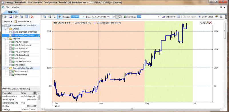
When the strategy is run it plots two price differences between the target index (instrument) and the tracking portfolio. The first price difference is reset after each rebalancing. The second price difference is reset only after the first rebalancing and shows how index (instrument) behavior is approximated by the tracking portfolio globally.

Genetic algorithm parameters are defined by the fields “Population size”, “Number of generations”, “Percent of Dominating Chromosomes”, “Percent of Elite” and “Percent of Mutated”. Their meaning is described above in the section ‘Method’.

Parameters of the index tracking genetic operators (see section Genetic Operators above) are defined by the following fields: “Shared Alleles Weight” is SharedAllelesWeight; “Number of Genes to Mutate at once” is NumberOfMutations; “Instrument vs Weight Mutations” is InstrumentVsWeight.

The size of a tracking portfolio is proportional to the transaction costs necessary to maintain it. So we should keep the portfolio as small as possible and discard negligible instruments. The field “Threshold Weight below which to discard Instrument” defines when the instrument is discarded from portfolio: the instrument j is discarded if the following is true:

Example: “DIA” is specified as the index ticker. As a ticker universe, all the available equities are chosen. Maximum portfolio size e.g. = 4. All the other parameters are set as default in the current configuration of the attached strategy. The tracker approximates the out-of-sample behaviour of DIA; the quality of approximation is dependent on market (of course) and quality of data (gaps etc.).

Below are the out of sample results from running a backtest in QuantOffice on the implementation of the Ravenpack strategy discussed here.

 

 

 

Background

The problem of optimal execution of large orders over a finite interval of time is not new. Interested readers may review the risk-adjusted cost minimization approach introduced by Almgren and Chriss (2001).

Generally speaking, the trader faces the problem of optimal execution of large orders because of limited supply-demand liquidity in the market(s). If the order size is small enough there is no such a problem and the whole volume could be executed immediately.

One of the approaches used by traders is to split the original order into a sequence of orders of smaller sizes and execute them within a required time interval.

Click here for the full paper.

As an ongoing exercise at Deltix, we seek out new sources of data, raw or derived, which may be useful in quantitative research and trading. We do this for a number of reasons. Firstly, handling new and different data types is a useful exercise with which to develop and road-test our software. Secondly, if we can seed ideas that our clients find useful and develop through to profitable trading strategies then it is just plain good business. Lastly, it satisfies our intellectual curiosity.

Ravenpack (www.ravenpack.com) is a data provider of news analysis services to institutions for use in quantitative trading. They recently released a data service of country sentiment factors. A research paper using these factors is available here. We decided to implement both Ravenpack’s country sentiment factors and their research paper on our Deltix Cloud Services (DCS) platform. The results are extremely interesting. Existing DCS users can download the strategy from the Deltix Developer Network (DDN), accessed from QuantOffice via the “Samples from DDN” button. New users can subscribe DCS and download the strategy here.

One of the paradoxes faced by quantitative researchers and traders is the granularity of data to use in the model back-testing phase. Putting aside using market depth data (order book Level 2, Level 3 data), the choice is in effect between bar data and tick data (trade, best bid/offer aka “BBO”). Bar data, is typically defined in terms of time duration, usually measured in minutes. The bar normally contains the open, high, low and closing (OHLC) quotes in the time period delineated by the bar. Traditionally, bar data has been used in preference to raw tick data because of much lower data density per time period, resulting in less storage and faster processing rates. Another benefit of bar data is that the regular and predictable nature of such data versus irregular (with respect to time) tick data means much simpler programming is required by the end user. However, inevitably, such benefits come at a cost of precision. For trading strategies generating signals infrequently, e.g. hourly or daily, there is minimum loss of precision. However, as signal generation increases in frequency, bars become less satisfactory for both signal generation and simulation of execution.

How then to combine the simplicity of bar data with the precision of tick data? Introducing “Enhanced Bars”.

Our researchers have designed a solution to this conundrum whereby we combine key statistics derived from the underlying tick data and extend the standard OHLC bars with additional attributes. (Hence, we use the term “extended bar” synonymously “enhanced bar”). For example, it is useful to know when the best bid and offer prices occur within the bar, and how many quotes are captured in the bar. Our enhanced bar is defined as (definition taken from our online documentation, Deltix Developer Network (DDN) at http://developer.deltixlab.com):

 

Field name	Field Type	Data Type
exchangeCode	Static	VARCHAR
originalTimestamp	Static	TIMESTAMP
open	Non Static	FLOAT
high	Non Static	FLOAT
low	Non Static	FLOAT
close	Non Static	FLOAT
volume	Non Static	FLOAT
currencyCode	Static	INTEGER
OpenTimeOffset	Non Static	INTEGER
HighTimeOffset	Non Static	INTEGER
LowTimeOffset	Non Static	INTEGER
CloseTimeOffset	Non Static	INTEGER
BestBid	Non Static	FLOAT
BestAsk	Non Static	FLOAT

 

For users of Deltix Cloud Services (DCS), you may download example strategies utilizing extended/enhanced bars at: http://dcs.developer.deltixlab.com/strategies/. DCS includes extended bar data at 10 second and 1 minute granularities.